The Preprocessing block prepares the data for consumption. During training, the data passes through five consecutive layers: Reshape, RandomWidth, RandomTranslation, RandomZoom, Resizing. However, during evaluation or production, the data only passes through the Reshape layer.
The Reshape layer reshapes the 2D tensor of size (n, 784) into (n, 28, 28, 1), n being the number of observations per batch. The RandomWidth layer scales the image along the x-axis by a random amount. The RandomTranslation layer translates the image to a random location. The RandomZoom layer zooms the image by a random amount. The Resizing layer resizes the image back to 28x28. The data is then sent off to be processed by the Convolutional and Singularity Extracting chains.
The Convolutional Chain is designed to learn and detect patterns that correspond to each digit. It, as illustrated below, is built with 11 building blocks: 3 convolutional blocks, 3 batch norm., 3 dropout layers, a global average pooling layer, and a redundant yet useful flattening layer.
The dropout layer discards some of the connections between layers, thus countering overfit. The batch normalization layer standardizes its inputs. The standardization of inputs helps the model learn faster as it does not have to spend numerous iterations adjusting each of the weights to account for extreme input values. The global average pooling layer maps the average of each spatial feature to a category confidence map which significantly reduces computational needs.

The flatten layer assures that all output from the chain is flattened.
The Convolutional Block is a series of sequentially connected convolutional, batch normalization, and max-pooling layers. During the instantiation of a block, we supply arguments upon which it generates and connects layers. Specifying the depth parameter causes the block to generate just as many "Convolution-Batch Norm" pairs, only leaving the last convolutional layer without a batch norm partner. If the pool argument is True, it generates a max-pooling layer of second degree; otherwise, it increases the strides of the last convolutional layer to 2. Below is a convolutional block with depth 2 and pooling enabled.
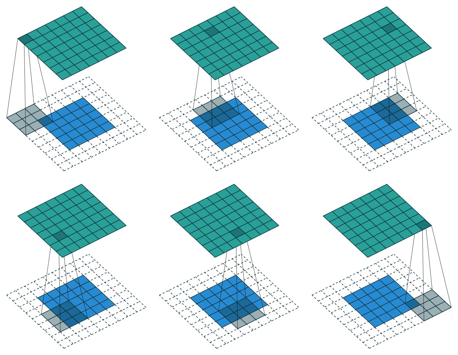
The convolutional layer applies a convolution operation (basically a dot product) on the input matrix using kernels. The weights of the kernels are inferred during training which allows the model to find useful repeating spatial patterns in the inputs. The animation below shows how the kernel (dark 3x3 area) passes above each input pixel (blue squares), applying a convolution operation to nearby pixels, thus computing the output (green matrix).

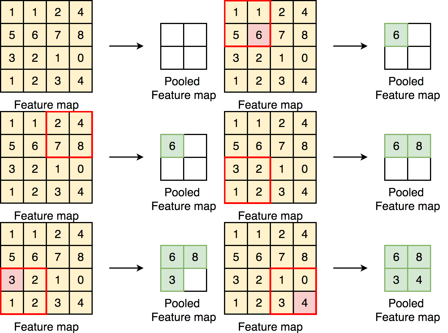
The max-pooling layer helps us reduce computational needs by down-sampling the input.

The Cognitive Block, as shown below, consists of concatenate, dense, batch norm, and dropout layers. The concatenate layer merges the outputs of the Convolutional and Singularity Extracting chains. The dense layers are just a bunch of linear functions with a touch of non-linearity (in this case, a leaky rectified linear unit, tanh, and softmax).